Matsubara correlation

In this example, we take the underdamped Brownian motion spectral density for a bath and calculate the Matsubara and non-Matsubara expoentials to express the correlation function as a sum of four exponents.

import numpy as np
from matsubara.correlation import (nonmatsubara_exponents,
                                   matsubara_zero_analytical,
                                   biexp_fit, sum_of_exponentials)
import matplotlib.pyplot as plt


coup_strength, bath_broad, bath_freq = 0.2, 0.05, 1.
tlist = np.linspace(0, 100, 1000)

# Zero temperature case beta = 1/kT
beta = np.inf
ck1, vk1 = nonmatsubara_exponents(coup_strength, bath_broad, bath_freq, beta)
corr_nonmats = sum_of_exponentials(1j*ck1, vk1, tlist)

# Analytical zero temperature calculation of the Matsubara correlation
mats_data_zero = matsubara_zero_analytical(coup_strength, bath_broad,
                                                                                   bath_freq, tlist)

# Fitting a biexponential function
ck20, vk20 = biexp_fit(tlist, mats_data_zero)

print("Non matsubara coefficients: ", ck1)
print("Non matsubara frequencies:", vk1)
print("Fitted matsubara coefficients: ", ck20)
print("Fitted matsubara frequencies:", vk20)
# Plotting the fit and non Matsubara parts
corr_fit = sum_of_exponentials(ck20, vk20, tlist)

fig, ax = plt.subplots(1, 2, figsize=(15, 5))

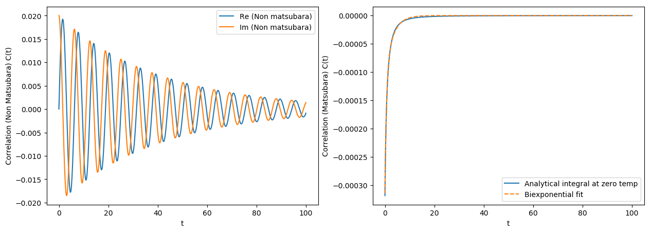
ax[0].plot(tlist, np.real(corr_nonmats), label="Re (Non matsubara)")
ax[0].plot(tlist, np.imag(corr_nonmats), label="Im (Non matsubara)")
ax[0].set_xlabel("t")
ax[0].set_ylabel("Correlation (Non Matsubara) C(t)")
ax[0].legend()

ax[1].plot(tlist, mats_data_zero, label="Analytical integral at zero temp")
ax[1].plot(tlist, corr_fit, "--", label="Biexponential fit")
ax[1].set_xlabel("t")
ax[1].set_ylabel("Correlation (Matsubara) C(t)")
ax[1].legend()
plt.show()