Hierarchical Eq. of Motion (HEOM)

We can calculate the dynamics of the spin-boson model at zero temperature with the Hierarchical Equations of Motion (HEOM) method in the following example.

import numpy as np
from matsubara.correlation import (sum_of_exponentials, biexp_fit,
                                   bath_correlation, underdamped_brownian,
                                   nonmatsubara_exponents, matsubara_exponents,
                                   matsubara_zero_analytical, coth)
from qutip.operators import sigmaz, sigmax
from qutip import basis, expect
from qutip.solver import Options, Result, Stats

from matsubara.heom import HeomUB

import matplotlib.pyplot as plt


Q = sigmax()
wq = 1.
delta = 0.
coup_strength, bath_broad, bath_freq = 0.2, 0.05, 1.
tlist = np.linspace(0, 200, 1000)
Nc = 9
Hsys = 0.5 * wq * sigmaz() + 0.5 * delta * sigmax()
initial_ket = basis(2, 1)
rho0 = initial_ket*initial_ket.dag()
omega = np.sqrt(bath_freq**2 - (bath_broad/2.)**2)
options = Options(nsteps=1500, store_states=True, atol=1e-12, rtol=1e-12)

# zero temperature case, renormalized coupling strength
beta = np.inf
lam_coeff = coup_strength**2/(2*(omega))

ck1, vk1 = nonmatsubara_exponents(coup_strength, bath_broad, bath_freq, beta)

# Ignore Matsubara
hsolver2 = HeomUB(Hsys, Q, lam_coeff, ck1, -vk1, ncut=Nc)
output2 = hsolver2.solve(rho0, tlist, options)
heom_result_no_matsubara = (np.real(expect(output2.states, sigmaz())) + 1)/2


# Add zero temperature Matsubara coefficients
mats_data_zero = matsubara_zero_analytical(coup_strength, bath_broad, bath_freq,
tlist)
ck20, vk20 = biexp_fit(tlist, mats_data_zero)
hsolver = HeomUB(Hsys, Q, lam_coeff, np.concatenate([ck1, ck20]),
                     np.concatenate([-vk1, -vk20]), ncut=Nc)
output = hsolver.solve(rho0, tlist, options)
heom_result_with_matsubara = (np.real(expect(output.states, sigmaz())) + 1)/2

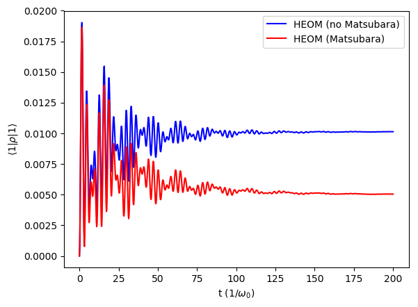
plt.plot(tlist, heom_result_no_matsubara, color="b", label= r"HEOM (no Matsubara)")
plt.plot(tlist, heom_result_with_matsubara, color="r", label=r"HEOM (Matsubara)")
plt.xlabel("t ($1/\omega_0$)")
plt.ylabel(r"$\langle 1 | \rho | 1 \rangle$")
plt.legend()
plt.show()