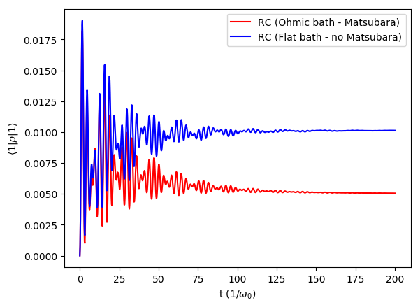
Reaction Coordinate (RC)

In this example, we calculate dynamics of the spin-boson model using a Reaction Coordinate (RC) approach corresponsing to two type of spectral densitities for the RC - flat bath (non Matsubara) and a Ohmic bath (Matsubara).

import numpy as np
from matsubara.correlation import (sum_of_exponentials, biexp_fit,
                                   bath_correlation, underdamped_brownian,
                                   nonmatsubara_exponents, matsubara_exponents,
                                   matsubara_zero_analytical, coth)
from qutip.operators import sigmaz, sigmax
from qutip import basis, expect, tensor, qeye, destroy, mesolve
from qutip.solver import Options, Result, Stats

from matsubara.heom import HeomUB

import matplotlib.pyplot as plt

Q = sigmax()
wq = 1.
delta = 0.
beta = np.inf
coup_strength, bath_broad, bath_freq = 0.2, 0.05, 1.
tlist = np.linspace(0, 200, 1000)
Ncav = 5

omega = np.sqrt(bath_freq**2 - (bath_broad/2.)**2)

# Try with omega = bath_freq
wrc = bath_freq
lam_renorm = coup_strength**2/(2*wrc)
lam2 = np.sqrt(lam_renorm)

# Construct the RC operators with a flat bath assumption for RC
sx = tensor(sigmax(), qeye(Ncav))
sm = tensor(destroy(2).dag(), qeye(Ncav))
sz = tensor(sigmaz(), qeye(Ncav))
a = tensor(qeye(2), destroy (Ncav))
options = Options(nsteps=1500, store_states=True, atol=1e-13, rtol=1e-13)        # Options for the solver.

Hsys = 0.5*wq*sz + 0.5*delta*sx + wrc*a.dag()*a + lam2*sx*(a + a.dag())
initial_ket = basis(2, 1)
psi0 = tensor(initial_ket, basis(Ncav,0))

#coup_strength of SD is 1/2 coup_strength used in ME
c_ops = [np.sqrt(bath_broad)*a]
e_ops = [sz, sm.dag(), a, a.dag(), a.dag()*a, a**2, a.dag()**2]
rc_flat_bath = mesolve(Hsys, psi0, tlist, c_ops, e_ops, options=options)
output = (rc_flat_bath.expect[0] + 1)/2.


# RC with a Ohmic spectral density. `c_ops` are calculated using
c_ops = []
wrc = bath_freq
groundval, gstate = Hsys.eigenstates()

bath_op_renorm = (a + a.dag())/np.sqrt(2*wrc)

for j in range(2*Ncav):
    for k in range(j, 2*Ncav):
        e_diff = groundval[k] - groundval[j]
        matrix_element = bath_op_renorm.matrix_element(gstate[j], gstate[k])
        rate = 2.*e_diff*bath_broad*(matrix_element)**2

        if np.real(rate) > 0. :
            c_ops.append(np.sqrt(rate) * gstate[j]* gstate[k].dag())

e_ops = [sz,]
rc_ohmic_bath = mesolve(Hsys, psi0, tlist, c_ops, e_ops,options=options)
output2 = (rc_ohmic_bath.expect[0] + 1)/2

plt.plot(tlist, output2, color="b", label="RC (Ohmic bath - Matsubara)")
plt.plot(tlist, output, color="r", label="RC (Flat bath - no Matsubara)")
plt.xlabel("t ($1/\omega_0$)")
plt.ylabel(r"$\langle 1 | \rho | 1 \rangle$")
plt.legend()
plt.show()