Positivity constrained fitting
An example on how to impose a constraint on the fit of the correlation functions so that positivity in the final pseudo-mode model is preserved.
import numpy as np
from matsubara.correlation import spectrum_matsubara, spectrum_non_matsubara, spectrum
from matsubara.correlation import (sum_of_exponentials, biexp_fit, biexp_fit_constrained,
bath_correlation, underdamped_brownian,
nonmatsubara_exponents, matsubara_exponents,
matsubara_zero_analytical, coth)
import matplotlib.pyplot as plt
bath_freq = 1.
bath_width = 1.0
coup_strength = 0.01
# Zero temperature
beta = np.inf
w = np.linspace(-3, 3, 1000)
tlist = np.linspace(0, 20, 1000)
#Fit without additional constraint:
mats_data_zero = matsubara_zero_analytical(coup_strength, bath_width,
bath_freq, tlist)
ck2, vk2 = biexp_fit(tlist, mats_data_zero)
# For a given exponential we got the following contribution
# to the power spectrum
def spectrum_matsubara_approx(w, ck, vk):
"""
Calculates the approximate Matsubara correlation spectrum
from ck and vk.
Parameters
==========
w: np.ndarray
A 1D numpy array of frequencies.
ck: float
The coefficient of the exponential function.
vk: float
The frequency of the exponential function.
"""
return ck*2*(vk)/(w**2 + vk**2)
def spectrum_non_matsubara_approx(w, coup_strength, bath_broad, bath_freq):
"""
Calculates the approximate non Matsubara correlation spectrum
from the bath parameters.
Parameters
==========
w: np.ndarray
A 1D numpy array of frequencies.
coup_strength: float
The coupling strength parameter.
bath_broad: float
A parameter characterizing the FWHM of the spectral density, i.e.,
the bath broadening.
bath_freq: float
The bath frequency.
"""
lam = coup_strength
gamma = bath_broad
w0 = bath_freq
gam = gamma/2.
om = np.sqrt(w0**2-gam**2)
return (lam**2/(2*om))*2*(gam)/((w-om)**2+gam**2)
sm1 = spectrum_matsubara_approx(w,ck2[0],-vk2[0])
sm2 = spectrum_matsubara_approx(w,ck2[1],-vk2[1])
snm = spectrum_non_matsubara_approx(w,coup_strength,bath_width,bath_freq)
total_spectrum_unconstrained = (sm1 + sm2 + snm)
#fix the fit with a cost function to remove negative parts of spectrum
#for a given frequency range
ck2c, vk2c = biexp_fit_constrained(tlist, mats_data_zero, w, coup_strength,
bath_width, bath_freq, weight=1.)
#check spectrum again
sm1 = spectrum_matsubara_approx(w,ck2c[0],-vk2c[0])
sm2 = spectrum_matsubara_approx(w,ck2c[1],-vk2c[1])
snm = spectrum_non_matsubara_approx(w,coup_strength,bath_width,bath_freq)
total_spectrum_constrained = (sm1 + sm2 + snm)
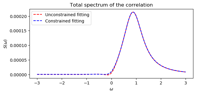
fig, ax1 = plt.subplots(figsize=(12, 7))
ax1.plot(w, total_spectrum_unconstrained, "--", color = "red", label="Unconstrained fitting")
ax1.plot(w, total_spectrum_constrained, "--", color = "b", label="Constrained fitting")
ax1.set_xlabel(r"$\omega$")
ax1.set_ylabel(r"$S(\omega)$")
ax1.legend()
ax1.set_title("Total spectrum of the correlation")
plt.show()
reconstructed_mats = sum_of_exponentials(ck2, vk2, tlist)
reconstructed_mats_constrained = sum_of_exponentials(ck2c, vk2c, tlist)
#compare original and new fit in terms of correlations
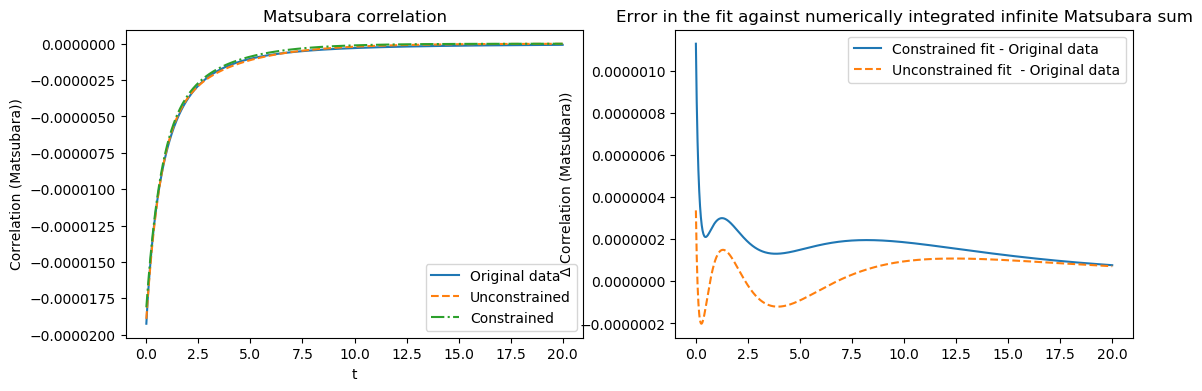
fig, [ax1, ax2] = plt.subplots(1, 2, figsize=(20, 7))
ax1.plot(tlist, mats_data_zero , label="Original data")
ax1.plot(tlist, reconstructed_mats,linestyle='--', label="Unconstrained")
ax1.plot(tlist, reconstructed_mats_constrained,linestyle='-.', label="Constrained")
ax1.set_ylabel("Correlation (Matsubara))")
ax1.set_xlabel("t")
ax1.legend()
ax2.plot(tlist, reconstructed_mats_constrained - mats_data_zero , linestyle='-',label="Constrained fit - Original data")
ax2.plot(tlist, reconstructed_mats - mats_data_zero , linestyle='--', label="Unconstrained fit - Original data")
ax2.set_ylabel(r"$\Delta$ Correlation (Matsubara))")
ax1.set_xlabel("t")
ax2.legend()
ax1.set_title("Matsubara correlation")
ax2.set_title("Error in the fit from numerical intergration of infinite Matsubara terms")
plt.show()